Series 04 — finale. This article unifies the device, state-space, and measurement viewpoints developed in the preceding three tutorials.
The first three articles answered three progressively harder questions. Two independently programmable retardances can generate arbitrary spatial polarization from a known fixed input. Polarization reachability does not necessarily imply reachability of the full complex vectorial state. Finally, two polarization evolutions with the same endpoints can acquire different geometric phases because their paths differ.
The missing final step is to place all three results inside one mathematical object. That object is neither a Stokes vector alone nor an isolated phase map. It is the complete complex Jones field
The result in one paragraph
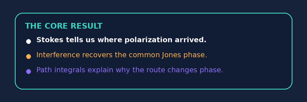
The Stokes vector specifies the polarization ray represented by a point on the Poincaré sphere, but it removes the common phase of the Jones vector. Coherent interferometry recovers that missing phase relative to a reference field. When a control parameter varies continuously, the Pancharatnam–Mukunda–Simon construction separates the endpoint phase from the local phase accumulated along the path, yielding a gauge-invariant geometric contribution. A defensible SLM experiment must therefore retain the complex fieldsand , reconstruct the Stokes trajectory, and measure a coherent phase reference. None of these three records can replace the other two.
1. Start with the full Jones device chain
For a nondepolarizing optical system, write every device in the physical order encountered by the beam:
The parameter may be an SLM grayscale value, a calibrated retardance, a wave-plate angle, propagation distance, a transverse coordinate, or an experimental scan index.
The output can be written as
This expression contains three distinct records:
- : optical intensity;
- : the normalized polarization state, defined only up to a common phase;
- : a common Jones phase defined relative to a chosen gauge or, experimentally, to a coherent reference.
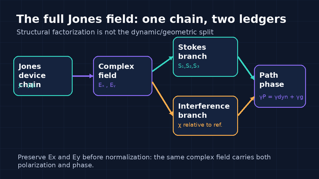
Figure 1. Preserve the complex fields before normalization. The same pair produces both the Stokes parameters and a phase relative to a coherent reference.
Saving only intensity discards relative and common phase. Saving only Stokes parameters discards common phase. Conversely, recording one interferometric projection does not by itself identify the polarization path or distinguish a path-dependent phase from ordinary optical-path drift.
2. Why the Poincaré sphere is missing one phase coordinate
For any normalized Jones state,
A point on the Poincaré sphere is therefore not one Jones vector. It is an equivalence class of vectors related by a common phase.
Geometrically, the sphere is the base space of polarization rays, while a phase fiber is attached to every point. The full normalized Jones state belongs to the corresponding spinor space. This fiber-bundle viewpoint provides a common origin for optical geometric phases and makes clear why polarimetry alone cannot recover them as coherent phases.
The practical translation is simple:
- the Stokes record answers where the polarization arrived;
- the interferometric record answers where the Jones vector lies on the phase fiber;
- the path record explains how the route contributes a geometric phase.
3. The factorization—and its limitation
For a lossless nondepolarizing device, the Jones matrix is unitary and may be factored as
with
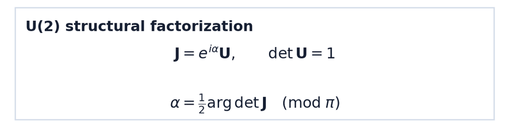
The scalar factor belongs to , whereas produces the associated rotation of the Stokes vector. The phase is defined modulo because the replacements and leave unchanged.
This is a structural factorization of a device matrix. It is not automatically the physical decomposition
The operator can contribute a state-dependent Pancharatnam phase when it acts on a particular input. A dynamic/geometric split additionally requires a specified continuous evolution or a calibrated generator. Reading only is therefore insufficient to identify every phase observed in an interferometer.
4. Six phase quantities that must remain separate
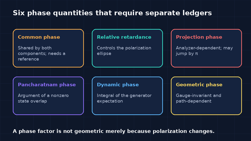
Figure 2. These quantities may appear in the same optical system, but they describe different operations or observables.
| Quantity | Definition or role | How it is obtained |
|---|---|---|
| Common Jones phase | A factor multiplying both Jones components | Coherent interference with a reference |
| Relative retardance | Phase difference between two polarization components or eigenmodes | Polarimetry or calibrated device model |
| Projection phase | Argument of | after an analyzer |
| Pancharatnam phase | for nonorthogonal states | |
| Dynamic phase | Integral of a specified evolution generator expectation | Continuous model or independent calibration |
| Geometric phase | Gauge-invariant remainder determined by the path | Kinematic integral, Bargmann product, or solid angle |
This series uses
If
then the convention-consistent relation is
Changing the convention, viewing direction, or sphere orientation changes several signs together. It is not valid to change one geometric-phase sign without updating the complete Jones–Stokes convention.
5. A complete SLM–QWP calculation
Take 45-degree linear input,
followed by an ideal SLM that modulates only the component,
The SLM matrix itself can be written as
Now place a quarter-wave plate with its fast axis at 45 degrees after the SLM. Using zero phase on the fast axis and a slow-axis retardance,
The output becomes
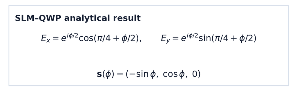
The bracketed vector is real, so the ideal output is linearly polarized with azimuth
Its normalized Stokes trajectory is
which lies on the equator of the Poincaré sphere.
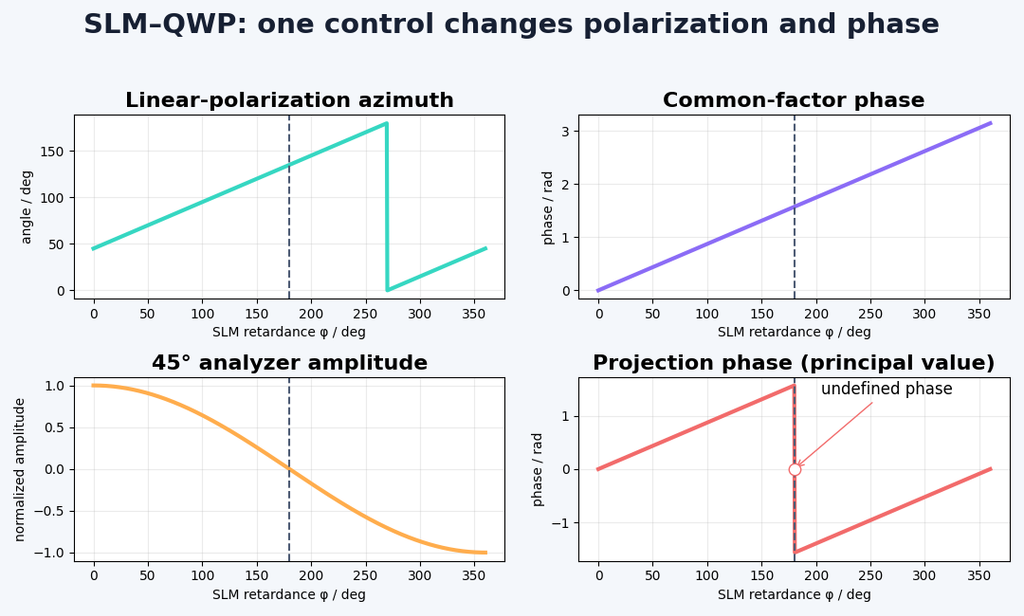
Figure 3. One SLM control parameter changes the polarization azimuth, a common factor in the chosen Jones representation, and the phase of a selected analyzer projection.
For a 45-degree analyzer ,
At , the projected amplitude vanishes. Its phase is undefined at that point and the principal value exhibits a jump across it. This is first a projection zero and phase singularity. It must not be relabeled as a geometric phase without a path-based calculation.
As runs from to , the Stokes vector completes the equator. With the convention and orientation fixed in this series, the enclosed solid angle is , giving a closed-path geometric phase of modulo . The common factor, spinor sign, local phase accumulation, and final interferometric phase must still be combined consistently.
6. The kinematic dynamic/geometric split
For a smooth normalized path whose endpoints are nonorthogonal, define the endpoint Pancharatnam phase as
The open-path geometric phase is
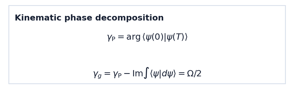
The endpoint term and the integral are individually gauge-dependent, but their combination is invariant under
If the evolution obeys
then
and
This point is experimentally important: a sequence of endpoint Jones matrices does not, by itself, determine a unique dynamic phase. The internal continuous realization or an independently calibrated device model must be supplied.
For a discrete SLM or wave-plate sequence, three numerical routes should be cross-checked:
- neighboring nonzero Jones overlaps;
- Bargmann products for triangles or polygons;
- a signed solid angle obtained by triangulating the Stokes path.
Orthogonal consecutive states require segmentation or an auxiliary reference because the argument of a zero overlap is undefined.
7. A decisive same-endpoint experiment
Choose horizontal polarization as the initial state and 45-degree linear polarization as the final state. Compare:
- Path A: the direct shortest geodesic from;
- Path B: a piecewise geodesic from through a circular pole , then to .
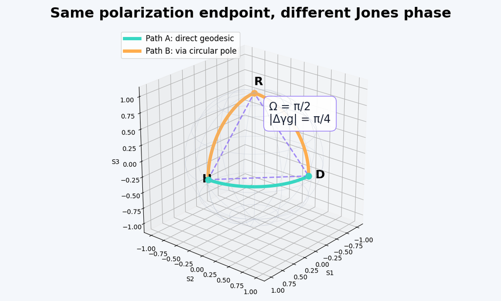
Figure 4. The final Stokes vectors are identical, but the closed loop formed by the two routes subtends a nonzero solid angle. The figure displays the magnitude; the sign depends on the specified vertex ordering and orientation.
The spherical triangle has solid-angle magnitude
and therefore
An ideal Stokes polarimeter reports the same endpoint for the two routes. A phase-stable interferometer referenced to the same field reports a fringe-phase difference. Reversing the traversal reverses the geometric-phase sign.
This experiment provides the cleanest operational meaning of the series finale: identical polarization endpoints do not imply identical Jones states.
The path can be synthesized with a universal wave-plate gadget such as QWP–HWP–QWP, or with calibrated SLM interactions. To isolate the geometric contribution, choose geodesic or parallel-transport segments when possible and independently measure residual dynamic and propagation phases.
8. Polarization-diverse coherent measurement
A single analyzer projection can vanish and create a phase blind spot. A stronger architecture separates the two Jones components and measures each against a matched reference.
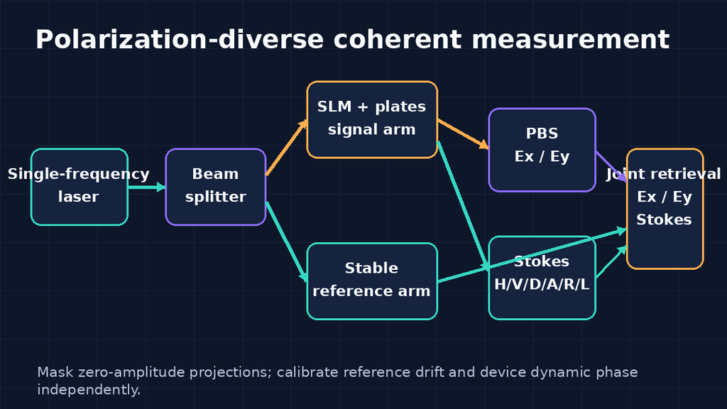
Figure 5. Proposed validation architecture. It is an authorial extension based on the cited theory, not an experiment already reported in the two SLM papers discussed earlier in the series.
The system contains:
- a single-frequency spatially filtered source;
- a splitter that creates signal and phase-stable reference arms;
- a calibrated SLM–wave-plate or multi-pass SLM path generator;
- a Stokes-analysis branch measuring ;
- a PBS that separates for coherent detection;
- phase-shifting or off-axis holographic reconstruction.
For four phase steps , the complex cross term in polarization channel is
After calibration against the reference amplitudes, recover the two complex signal components. The same dataset then yields intensity, relative retardance, Stokes parameters, common phase relative to the reference, and path-dependent phase diagnostics.
Required controls include:
- masking pixels with near-zero signal or reference amplitude;
- phase unwrapping only inside connected valid regions;
- reference-arm drift correction;
- SLM grayscale-to-retardance calibration;
- polarization matching in both interferometric channels;
- checks for diattenuation, zero-order leakage, crosstalk, and registration error.
9. Incorporating the framework into SLM optimization
Rather than hiding every discrepancy inside one scalar objective, record at least four terms:
Here is a diagnostic or regularizer for dynamic and geometric contributions. It need not always be a control target. If the application only requires the final full Jones field, the amplitude, polarization, and common-phase losses already specify that endpoint. A geometric-phase term becomes useful when different control routes must be compared, when path sensitivity is itself functional, or when phase robustness under path reversal is being tested.
The fourth orthogonal interaction in the 2020 theoretical model directly restores missing common-phase reachability. A polarization path may contribute geometric phase, but it is not the sole reason the fourth interaction works. Calling the full added capability “pure geometric-phase control” would be inaccurate.
10. Where the Jones framework stops
The treatment above assumes a monochromatic or narrowband, coherent, fully polarized, nondepolarizing field that can be represented locally by a deterministic Jones matrix.
If an element has loss and diattenuation but remains nondepolarizing, use a polar decomposition such as
where is positive Hermitian and is unitary. The path on the Poincaré sphere then need not be a pure rotation, and nonunitary geometric-phase definitions require additional care.
If the system truly depolarizes, averages over fluctuating scattering paths, or contains partially coherent mixtures, a single Jones vector is insufficient. The appropriate description moves to a coherency matrix, Mueller matrix, or mixed-state geometric phase. Pure-state solid-angle formulas must not be applied uncritically to those data.
11. Closing the four-article series
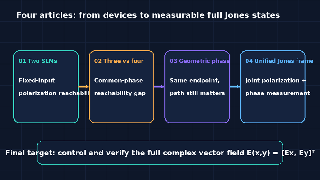
Figure 6. The series progresses from fixed-input polarization synthesis to full Jones-state reachability, path-dependent phase, and joint coherent measurement.
- Article 01: two independent retardances provide polarization reachability for a known input;
- Article 02: polarization reachability is not full Jones-state reachability;
- Article 03: the route can matter even when polarization endpoints agree;
- Article 04: the same record unifies calculation, control, and measurement.
The entire series can be condensed into one statement:
The Stokes vector tells us where polarization arrived, coherent interference tells us the remaining common Jones phase, and geometric phase records how the state reached that endpoint.
References
- F. Kenny et al., “Complete polarization and phase control for focus-shaping in high-NA microscopy,” Optics Express 20, 14015–14029 (2012). doi:10.1364/OE.20.014015
- Q. Hu et al., “Arbitrary vectorial state conversion using liquid crystal spatial light modulators,” Optics Communications 459, 125028 (2020). doi:10.1016/j.optcom.2019.125028
- S. Pancharatnam, “Generalized theory of interference, and its applications. Part I,” Proceedings of the Indian Academy of Sciences A 44, 247–262 (1956). doi:10.1007/BF03046050
- J. Samuel and R. Bhandari, “General Setting for Berry’s Phase,” Physical Review Letters 60, 2339–2342 (1988). doi:10.1103/PhysRevLett.60.2339
- R. Simon and N. Mukunda, “Minimal three-component SU(2) gadget for polarization optics,” Physics Letters A 143, 165–169 (1990). doi:10.1016/0375-9601(90)90732-4
- N. Mukunda and R. Simon, “Quantum Kinematic Approach to the Geometric Phase. I. General Formalism,” Annals of Physics 228, 205–268 (1993). doi:10.1006/aphy.1993.1093
- C. Cisowski, J. B. Götte, and S. Franke-Arnold, “Geometric phases of light: Insights from fiber bundle theory,” Reviews of Modern Physics 94, 031001 (2022). doi:10.1103/RevModPhys.94.031001
- D. Kestner and A. Kostinski, “Simple formula for the Jones product and the Pancharatnam connection in optics,” Physical Review A 109, 023517 (2024). doi:10.1103/PhysRevA.109.023517
Series navigation
- 01 — Two SLMs for spatial polarization and common-wavefront control
- 02 — Three versus four SLM interactions: polarization reachability is not full-state reachability
- 03 — Same endpoints, different paths: Pancharatnam and geometric phase
- 04 — One Jones framework for polarization endpoints and phase paths
The offline interactive companion is located at tools/jones-stokes-phase-unified-en.html.