---

Series cover. The path motif is an original explanatory graphic rather than a figure reproduced from a cited paper.

Series 03 — phase beyond the polarization endpoint

The previous article identified an apparent paradox: two fields can occupy exactly the same point on the Poincaré sphere while their Jones vectors differ by $(\pi/2)$, or by any other common phase.

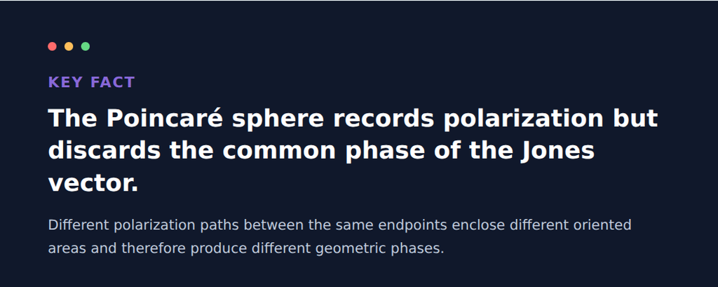
There is no contradiction. The Poincaré sphere records polarization, not the global phase of a Jones vector. Moreover, even when two polarization evolutions share the same initial and final states, their different paths can accumulate different geometric phases.

This article connects the Pancharatnam relative phase, open-path geometric phase, Bargmann invariants, and an experimentally measurable interferometric phase. It is a tutorial synthesis, not a reconstruction of one paper’s experimental apparatus.

The result in one paragraph

Multiplying a Jones vector by $(e^{i\beta})$ leaves every Stokes parameter unchanged. The phase between two nonorthogonal polarization states can nevertheless be defined by the argument of their complex inner product. For a continuous evolution, subtracting the path-dependent local phase accumulation from the endpoint Pancharatnam phase gives a gauge-invariant geometric phase. With a specified Stokes convention and sphere orientation, this phase equals half the oriented solid angle enclosed after geodesic closure. Polarimetry alone cannot measure it: an experiment needs both a Stokes-analysis channel and a coherent phase-reference channel.

1. Six phase concepts that should not be merged

Term	What it describes	Typical measurement or calculation
Common or global Jones phase	A factor multiplying both Jones components	Interference with a phase reference
Dynamic phase	Phase accumulated from propagation or a device Hamiltonian/retardance process	Optical-path or calibrated device model
Relative retardance	Phase difference between two eigenpolarizations	Polarimetry or retarder calibration
Projection phase	Argument of a field after projection onto an analyzer state	Complex projection amplitude
Pancharatnam relative phase	Relative phase between two nonorthogonal polarization states	$\arg( A)$
Geometric phase	Gauge-invariant phase determined by a path in state space	Path integral, Bargmann product, or oriented solid angle

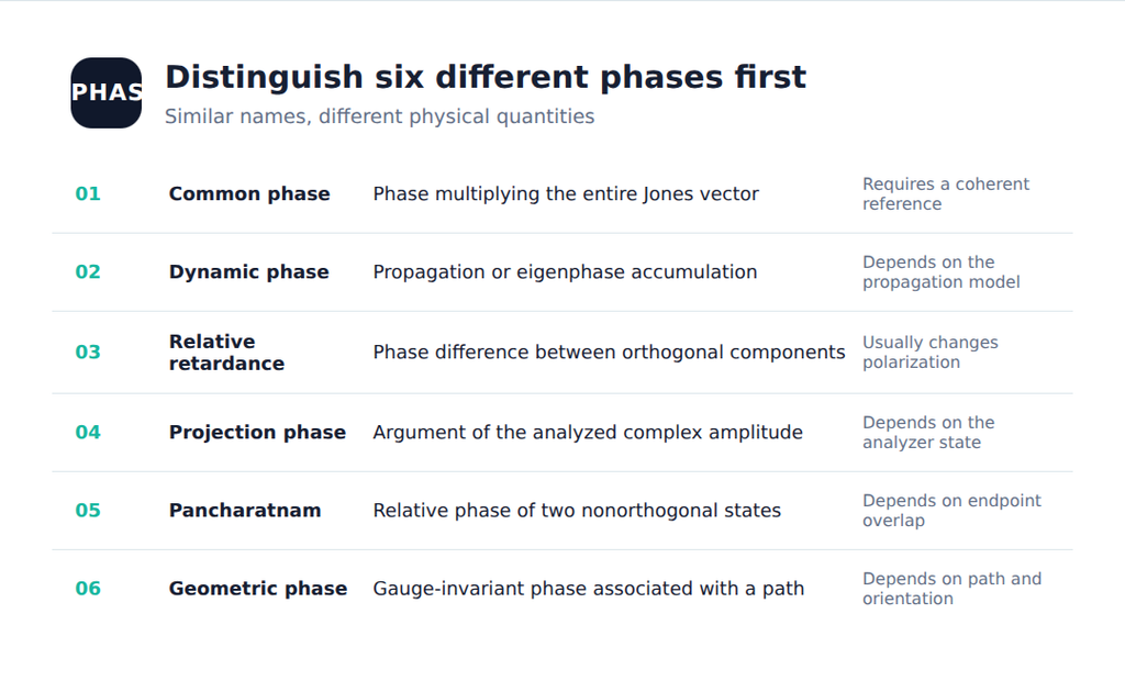
Figure 1. Six quantities that are often called “phase” but refer to different observables or decompositions.

A phase appearing in an optical system is not automatically a geometric phase. The reference state, propagation path, sign convention, and measurement must be specified.

2. Why the Poincaré sphere removes the global phase

For any normalized Jones state $(|\psi\rangle)$,

One point on the Poincaré sphere therefore represents an entire equivalence class of Jones vectors that differ only by a common phase.

For example, $([0,1]^T)$ and $(i[0,1]^T)$ are the same vertical polarization state, but they produce a $(\pi/2)$ phase difference when interfered with the same coherent reference.

That phase may be imposed directly by an SLM or accumulated through ordinary propagation. It is first a common or dynamic phase; it does not become geometric merely because the polarization is represented on a sphere.

3. The Pancharatnam connection

For two normalized, nonorthogonal polarization states $(|A\rangle)$ and $(|B\rangle)$, the Pancharatnam relative phase is

The two states are “in phase” in Pancharatnam’s sense when their inner product is real and positive. Along a continuous path, choosing adjacent states to remain locally in phase defines parallel transport.

The subtlety is global: every infinitesimal step can satisfy the local in-phase condition, yet a closed path can return to the initial polarization with a nonzero residual phase. That residual is geometric.

When two states are orthogonal, their inner product is zero and its argument is undefined. A unique Pancharatnam phase cannot be assigned directly. One must introduce an intermediate reference, split the path, or take a carefully defined limit.

4. Open-path geometric phase

This series uses the Stokes convention

The orientation of the Poincaré sphere and the direction of path traversal are also fixed. Under the convention used here, the oriented-solid-angle relation is $(\gamma_g=\Omega/2)$. Reversing the $(S_3)$ convention or sphere orientation reverses the sign consistently.

For a smooth normalized path $(|\psi(s)\rangle)$ from $(|\psi_i\rangle)$ to $(|\psi_f\rangle)$, the gauge-invariant open-path geometric phase is

The endpoint term and the path integral can each change when the Jones-vector phase convention is changed, but their combination does not.

When the endpoints are nonorthogonal, the physical path can be closed by the shorter geodesic. If the resulting oriented solid angle is $(\Omega)$, then, with the convention adopted here,

For antipodal endpoints, the shortest geodesic is not unique. The closure rule must then be supplied explicitly.

5. Same endpoints, two different paths

Choose

These are 45° and 90° linear polarizations. Compare:

• a direct shortest-geodesic path from $(A)$ to $(C)$;
• a detour through the circular state

With $(S_3=2\operatorname{Im}(E_xE_y^*))$, this $(B)$ lies at the positive $(S_3)$ pole. The direct path encloses no area with its geodesic closure. The detour encloses an oriented spherical triangle.

The three-state Bargmann invariant gives

The corresponding oriented solid angle is $(-\pi/2)$, so $(\Omega/2=-\pi/4)$, consistent with the Bargmann result.

Reversing the path, choosing the opposite circular pole, or reversing the Stokes convention changes the sign. The magnitude of the phase difference in this example remains $(\pi/4)$.

The Bargmann product is useful because it is invariant when $(|A\rangle)$, $(|B\rangle)$, and $(|C\rangle)$ are independently multiplied by arbitrary phase factors. It is therefore an effective cross-check between Jones algebra and sphere geometry.

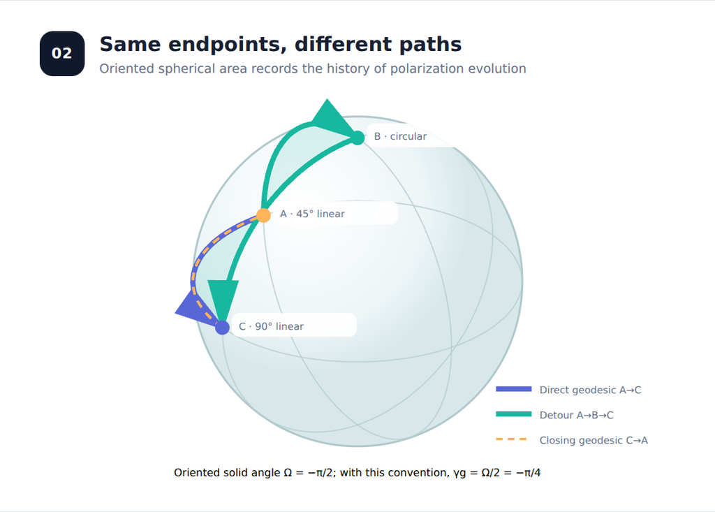
Figure 2. The two paths share endpoints but enclose a nonzero oriented solid angle after geodesic closure.

6. Three common sources of false “geometric phase” claims

A $(\pi)$ jump after a linear analyzer

After projection onto a linear analyzer, a real field amplitude can change sign. Its principal argument then jumps by $(\pi)$. This is a projection-sign change and is not, by itself, a Pancharatnam–Berry phase.

The retardance of a wave plate

A quarter-wave plate introduces a $(\pi/2)$ relative retardance and a half-wave plate introduces $(\pi)$. Retardance changes polarization, but the retardance value is not automatically equal to the geometric phase accumulated along a chosen state-space path.

The $(\pm2\theta)$ phase of a rotated half-wave plate

For circularly polarized input, an ideal half-wave plate with axis angle $(\theta)$ flips the handedness and introduces a geometric phase proportional to $(\pm2\theta)$. The sign depends on the handedness, time convention, propagation direction, and fast-axis convention. The convention-independent statement is that opposite incident handednesses acquire opposite signs and that the angular dependence is doubled.

7. An SLM-plus-QWP example

Consider 45° linear input passing through an SLM that modulates only the $(x)$ component by $(\phi_x)$, followed by a quarter-wave plate whose fast axis is at 45°. Take the fast-axis phase as zero and the slow-axis delay as $(\pi/2)$. The output can be written as

The bracketed components are real, so the ideal output remains linearly polarized. Its azimuth is

while the chosen Jones representation contains a common factor $(e^{i\phi_x/2})$.

This decomposition does not prove that every interferometrically measured phase equals $(\phi_x/2)$, or that $(\phi_x/2)$ is purely geometric. Projection amplitudes can cross zero and introduce additional $(\pi)$ branch jumps. A measurable phase must be defined relative to a specified reference field or analyzer state.

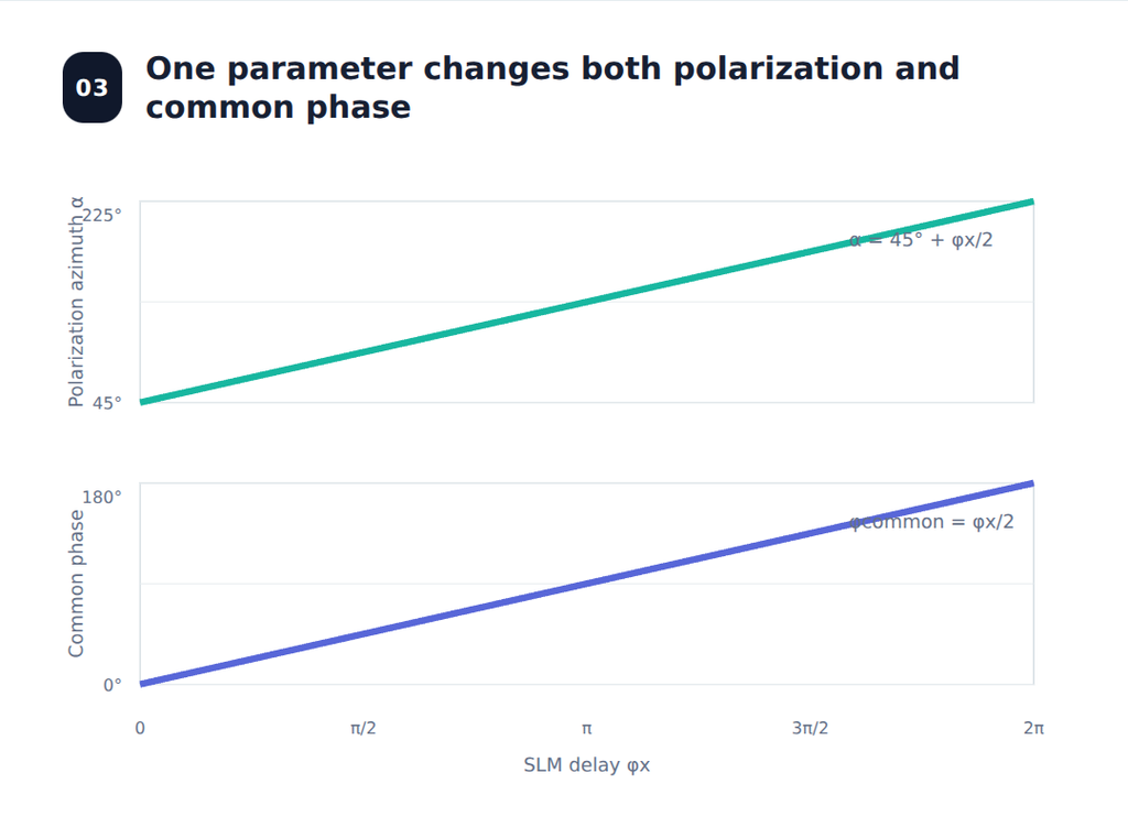
Figure 3. In the ideal SLM-plus-QWP example, one control parameter changes both the linear-polarization azimuth and a common phase factor.

8. Three numerical routes to the same geometric phase

A simulation that stores the Jones state after every optical element can evaluate geometric phase in three complementary ways:

1. Discrete Pancharatnam accumulation: multiply or sum the phases of neighboring complex overlaps along the path.
2. Bargmann invariants: use products of overlaps for triangular or polygonal paths.
3. Oriented solid angle: triangulate the closed path on the Poincaré sphere and add the signed areas.

The methods should agree only after the Jones convention, state ordering, handedness convention, and sphere orientation have been made consistent.

If two implementations differ by a sign, check:

• the definition of $(S_3)$;
• the viewing and propagation directions;
• the order of the spherical vertices;
• the handedness assigned to the circular poles;
• whether the path crosses an orthogonal state or a phase singularity.

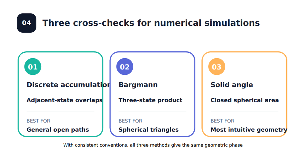
Figure 4. Discrete overlap accumulation, the Bargmann invariant, and oriented solid angle provide complementary numerical checks.

9. How to measure the phase experimentally

This section is a proposed validation architecture based on the cited theory. It is not copied from a single reference experiment.

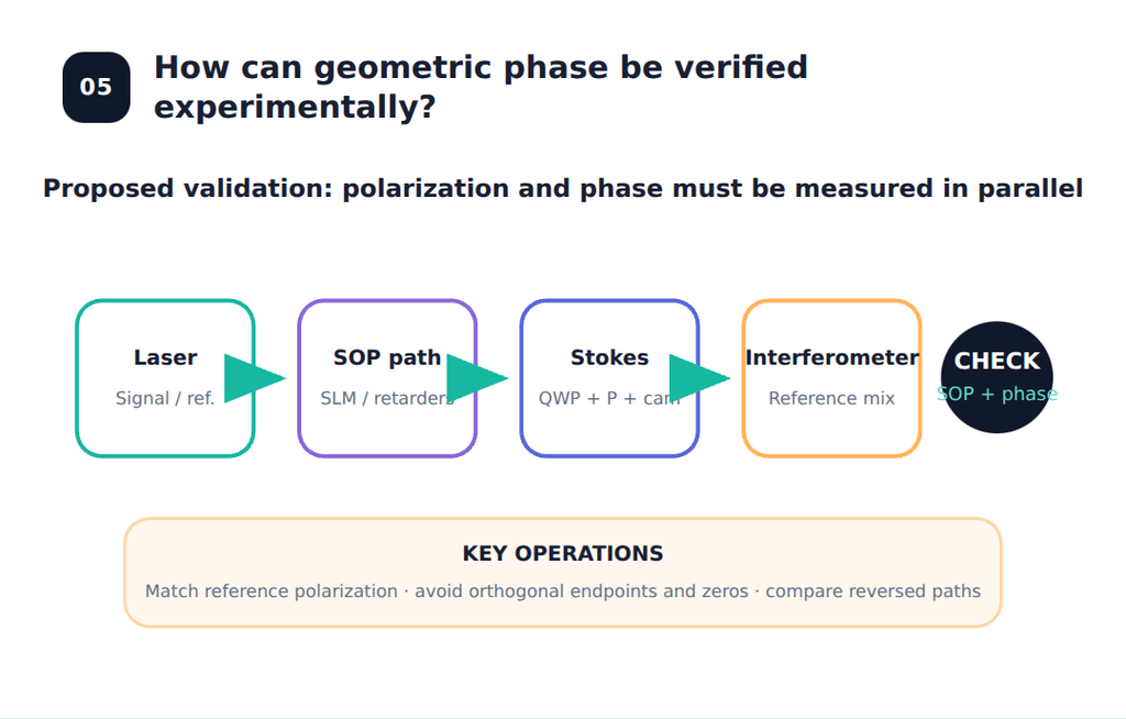
Figure 5. Proposed validation architecture. This dual-channel system is an authorial extension, not an experimental result reported in the two cited SLM papers.

1. Coherent source and beam splitting

A single-frequency laser is spatially filtered and divided into a signal arm and a stable reference arm. The reference arm includes adjustable delay and polarization matching.

2. Polarization-path generator

The signal arm passes through programmed SLM regions, quarter- and half-wave plates, or a multi-pass SLM system. These elements generate a prescribed open or closed path on the Poincaré sphere.

3. Stokes-analysis channel

A rotating quarter-wave plate and linear polarizer, or an equivalent full-Stokes polarimeter, measures the polarization state at each discrete step. This channel answers: “Where is the state on the sphere?”

4. Interferometric channel

The signal is projected onto a polarization component that has nonzero overlap with the reference. Off-axis holography or phase-shifting interferometry then recovers the complex phase. This channel answers: “What common phase remains outside the Stokes description?”

Both channels are required. Polarimetry alone cannot recover the global Jones phase, while interferometry alone cannot distinguish a polarization-path contribution from an ordinary optical-path drift.

Critical experimental conditions include:

• nonzero overlap between the selected signal projection and the reference polarization;
• rejection of phase estimates where the signal amplitude is near zero;
• avoidance or explicit treatment of orthogonal-state crossings;
• dynamic-phase controls based on reverse paths, complementary paths, or independent calibration;
• sufficient temporal and mechanical stability of the reference arm.

10. What this tutorial adds—and what it does not claim

This article does not propose a new geometric-phase theory. Its contribution is organizational:

• it connects the Pancharatnam inner-product definition to an open-path, gauge-invariant expression;
• it connects the Bargmann invariant to the oriented area on the Poincaré sphere;
• it separates common, dynamic, projection, and geometric phases in an SLM system;
• it gives a measurement architecture that combines Stokes polarimetry with coherent interferometry.

The proposed dual-channel experiment and the suggested closed-loop extensions are authorial extrapolations from the literature, not experimental results of the cited SLM papers.

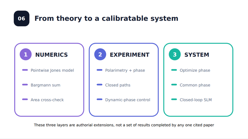
Figure 6. A three-layer extension from numerical cross-checks to dual-channel measurements and closed-loop calibration. These are proposed extensions rather than completed results of a single cited paper.

11. Returning to the four-interaction SLM system

The phase accumulated by a multi-SLM system generally contains several contributions: programmed component phases, relative retardances, ordinary propagation phase, fixed device offsets, and possibly a path-dependent geometric phase.

The fourth orthogonal SLM interaction in the 2020 model directly restores the missing controllable common-phase range. The geometric phase of the polarization path may contribute to the total, but it is not the whole reason the fourth interaction works. Calling the added capability “geometric-phase control” without this separation would be inaccurate.

Takeaway

The Poincaré sphere tells us whether the polarization endpoint is correct. It does not tell us whether the full Jones vector—including the phase relative to a reference—is correct. Different routes between the same polarization endpoints can add different geometric phases, and a defensible experiment must measure both the path in polarization space and the coherent phase.

References

1. S. Pancharatnam, “Generalized theory of interference, and its applications. Part I. Coherent pencils,” Proceedings of the Indian Academy of Sciences, Section A 44, 247–262 (1956). https://doi.org/10.1007/BF03046050
2. M. V. Berry, “The adiabatic phase and Pancharatnam’s phase for polarized light,” Journal of Modern Optics 34, 1401–1407 (1987). https://doi.org/10.1080/09500348714551321
3. J. Samuel and R. Bhandari, “General Setting for Berry’s Phase,” Physical Review Letters 60, 2339–2342 (1988). https://doi.org/10.1103/PhysRevLett.60.2339
4. J. C. Gutiérrez-Vega, “Pancharatnam–Berry phase of optical systems,” Optics Letters 36, 1143–1145 (2011). https://doi.org/10.1364/OL.36.001143
5. Q. Hu, Y. Dai, C. He, and M. J. Booth, “Arbitrary vectorial state conversion using liquid crystal spatial light modulators,” Optics Communications 459, 125028 (2020). https://doi.org/10.1016/j.optcom.2019.125028